meshBDD

A plant is a collection of similar components repeated many times (e.g. thousands of leaves). The most efficient way to store a plant into a file is to use reference meshes that describe the average geometry of a given component (e.g. a leaf or an internode), and then to transform this reference mesh to match precisely the geometry of each component. This method reduce the amount of data written in the .opf file because the geometry of each component is only stored in a 4*3 transformation matrix instead of a data heavy mesh. This matrix is then used to transform the reference mesh to match the geometry of a given component.

Hence, the meshBDD node of the .opf file lists all the reference meshes used to build the plant geometry. Here is the structure of the meshBDD from our example. Each reference mesh is represented by a mesh node with a given id, here we have three meshes with id 1, 2 and 0 respectively:

[...]
    <meshBDD>
            <mesh name="" shape="" Id="1" enableScale="true" >
              [...]
            </mesh>
            <mesh name="" shape="" Id="2" enableScale="false" >
          [...]
        </mesh>
          <mesh name="" shape="" Id="0" enableScale="false" >
            [...]
          </mesh>
    </meshBDD>
[...]

Each mesh node lists itself five information:
- the points coordinates as a vector of the form x1 y1 z1 x2 y2 z2 ...;
- the normal coordinates as a vector of the same form and order than the points;
- the texture coordinates (textureCoords) as a vector of the form u1 v1 u2 v2 ...;
- and the faces, listing face nodes, each containing a vector of 3 integers referring to the points index used to build a face. Point indices are written as i1 i2 i3. The preferred way for a face is to be a triangle (i.e. reference 3 points).

Here are more details about the first mesh:

        <mesh name="" shape="" Id="1" enableScale="true" >
            <points>
                0.10162586  -0.0012269035   -0.0    0.3519142   0.22452335  0.03067259  [...]
            </points>
            <normals>
                -0.17780079 -0.25352615 0.9508477   -0.17780079 -0.25352615 0.9508477   [...]
            </normals>
            <textureCoords>
                0.49726775  -0.38636366 0.010928948 0.003787874 0.0 0.46590912  [...]
            </textureCoords>
            <faces>
                <face Id="0">
                    0   2   4
                </face>
                <face Id="1">
                    0   4   3
                </face>
                <face Id="2">
                    4   8   6
                </face>
                [...]
            </faces>
        </mesh>

materialBDD

The materialBDD is used to declare the material properties for visualization purposes. This node is not used by ARCHIMED-φ, but is still mandatory to follow the .opf standard. It is used when rendering the .opf in e.g. XPlo.

The materialBDD is rather short. It lists material nodes that declare the optical properties of each reference node: the emission, ambient, diffuse, specular and shininess.

The materialBDD of our example is as follows:

[...]
    <materialBDD>
        <material Id="1">
            <emission>0.0   0.0 0.0 0.0 </emission>
            <ambient>1.0    0.0 0.0 1.0 </ambient>
            <diffuse>1.0    0.0 0.0 1.0 </diffuse>
            <specular>1.0   0.0 0.0 1.0 </specular>
            <shininess>10.0 </shininess>
        </material>
        <material Id="0">
            <emission>0.0   0.0 0.0 0.0 </emission>
            <ambient>1.0    0.8901961   0.0 1.0 </ambient>
            <diffuse>1.0    0.8901961   0.0 1.0 </diffuse>
            <specular>1.0   0.8901961   0.0 1.0 </specular>
            <shininess>10.0 </shininess>
        </material>
    </materialBDD>
[...]

Note that each material has an Id. This id can be different to the one provided in the meshBDD (see next paragraph). It is used to link the material to the mesh from the meshBDD by its Id.

Each material property (e.g. emission) stores a vector of 4 values for the red, green, blue, and alpha value ([0-1]).

shapeBDD

The shapeBDD is used to build a shape. A shape is an object that stores a mesh and a material. In other words, it is used to link each mesh to its material properties. Using shape is very powerful because it allows to recycle information whenever possible. For example different component types can have a different reference mesh, but share the same material properties. In this case, no need to create two identical material properties, we can just reference the same material instead when building the shape.

Here is the shapeBDD of our example:

[...]
    <shapeBDD>
        <shape Id="1">
            <name> Mesh1</name>
            <meshIndex>1</meshIndex>
            <materialIndex>1</materialIndex>
        </shape>
        <shape Id="2">
            <name> Mesh2</name>
            <meshIndex>2</meshIndex>
            <materialIndex>0</materialIndex>
        </shape>
        <shape Id="0">
            <name> Mesh0</name>
            <meshIndex>0</meshIndex>
            <materialIndex>0</materialIndex>
        </shape>
    </shapeBDD>
[...]

It lists 3 different shapes, each with a different reference mesh and material.

attributeBDD

Any kind of additional attributes (read “data”) can be attached to a topology node (i.e. decomp, follow and branch, see next paragraph). The attributeBDD is used to define the attribute name and class, i.e. data type, integer, float, string, or AMAPStudio custom keyword (e.g. Centimetre).

Here is the attributeBDD from our example:

[...]
    <attributeBDD>
        <attribute name="XX" class="Double"/>
        <attribute name="YY" class="Double"/>
        <attribute name="ZZ" class="Double"/>
        <attribute name="FileName" class="String"/>
        <attribute name="Length" class="Centimetre"/>
        <attribute name="Width" class="Centimetre"/>
        <attribute name="XEuler" class="Double"/>
    </attributeBDD>
[...]

It declares seven optional attributes that can be optionally attached to a topology node. These attributes are generally computed by a software and attached to the .opf. For example ARCHIMED-φ uses attributes to attach simulation outputs to .opfs from the scene, e.g. the intercepted PAR of each component. These attributes are handy for visualization purposes.

topology

The topology node is used to describe the relational connection between the different components of a plant, i.e. the organization of the plant. The components used are a natural decomposition of the plant, i.e. an internode or a leaf that are used to decompose the plant in metamers, and not an artificial decomposition such as a set of 10 cm long sections of axes.

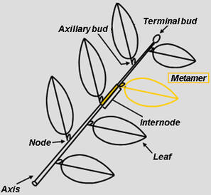
The leafy axis resulting from a succession of phytomers (or metamers) arising from apical bud growth and development. Drawing D. Barthélémy, CIRAD. Source

The description follows the rules of the widely used Multi-scale Tree Graph (MTG). Please read the article from Godin and Caraglio (1998) for a nice introduction to the concept.

But the topology node of the .opf enhances this concept by adding further attributes to each component, allowing a close coupling between the plant topology and geometry.

From Godin et al. (1999) Topology deals with the physical connections between plant components, while geometry includes the shape, size, orientation and spatial location of the components.

For example, each component to be rendered in 3D has a shapeIndex that points to the reference shape used to build the geometry of the component, and a geometry node that stores the transformation matrix applied to the reference mesh to compute the geometry of the component.

The topology is built by a succession of components, and the link between them is described using three main keywords:
- follow, for a succession of growth units created by apical meristems;
- branch for a ramification;
- decomp, for a decomposition, e.g a reiteration;

Here is the topology from our example file, without the details:

[...]
    <topology class="Scene" scale="0" id="3">          # -> instantiate the topology with a scene (scale 0)
        <decomp class="Individual" scale="1" id="2">     # -> instantiate an individual plant (scale 1)
          [...]
            <decomp class="Axis" scale="2" id="4">         # -> instantiate the base axis of the plant
              [...]
                <decomp class="Internode" scale="6" id="5">  # -> Start building the plant: first internode
                  [...]
                    <branch class="Leaf" scale="2" id="6">     # -> The 1st internode bears a leaf, branched to it
                      [...]
                    </branch>
                </decomp>
                <follow class="Internode" scale="6" id="10"> # -> The 2d internode follows the 1st internode
                  [...]
                    <branch class="Leaf" scale="2" id="11">    # -> The 2d leaf is branched into the 2d internode
                      [...]
                    </branch>
                </follow>
            </decomp>
        </decomp>
    </topology>
[...]

We can build the topology of our plant only by using the three keywords provided by the MTG method. This method is very powerful and is sufficient to build any topology configuration, from very simple plants to the most complex ones.

We see that each component is delimited by how it is connected to the previous one, and each one has also a class, a scale and an id. The scale is not very important for our purposes, but other two are:

• The class is used to declare a component type. This type can be anything, e.g. a leaf or an internode, but also a young_leaf and an old_leaf. The class is especially important in ARCHIMED-φ (compared to AMAPStudio) because it is then used to associate particular models and parameter values to each component type. We will see that later in the documentation about the models.

• The id is used as a unique identifier for the components. It helps us find e.g. a particular leaf in the whole plant.

geometry

As said previously, the geometry of the plant is the shape, size, orientation and spatial location of the components. It is defined by linking several information together: the reference shape declared earlier (see shapeBDD paragraph), and a transformation matrix given as an attribute to each component of the topology.

The transformation matrix is declared in a geometry node. This node also declares the shapeIndex to point to the reference shape to use, and two nodes called dUp and dDwn used for mesh tapering (e.g. make a cone from a cylinder). The geometry of the first leaf from our example .opf file is as follows:

[...]
  <branch class="Leaf" scale="2" id="6"> # -> declare a component (type: Leaf), branched to the previous component
    <Length>10.0</Length>                # -> Add optional attribute Length
    <Width>6.0</Width>                   # -> Add optional attribute Width
    <geometry class="Mesh">              # -> Add a geometry node
      <shapeIndex>1</shapeIndex>         # -> The shape 1 will be used as reference
        <mat>                              # -> The shape 1 will be transformed using this matrix
          8.6602545 0.0 -0.5    -1.7484555E-7
            0.0 1.0 0.0 0.0
            5.0 0.0 0.86602545  4.0
        </mat>
        <dUp>6.0</dUp>                     # -> Add tapering to the upper part of the shape
        <dDwn>6.0</dDwn>                   # -> Add tapering to the lower part of the shape
    </geometry>
  </branch>
[...]

The transformation matrix is an homogeneous matrix reduced to a 4*3 matrix because the 4th row of the matrix is always the same: [0 0 0 1]. Please read this wonderful resource for a nice introduction to homogeneous coordinates, translation, scaling and rotation. This method allows to reduce the data needed to describe the geometry in the .opf for fast IO and low disk space usage.

Further ressources

See this online course on the greenlab website and the AMAPStudio documentation for more information.